🚍 The Transformer Architecture
My notes draw extensively from the visual explanations and illustrations provided in the excellent blog post The Illustrated Transformer
1. Create three vectors from each of the encoder's input vectors (e.g. embedding of each word)
What is the Transformer?
- The paper introduces a novel SOTA architecture for machine translation applications, the Transformer model
- This model surpasses the existing best results at a fraction of the training costs required by the best models
- This achievement is possible due to the use of attention mechanisms only, which enable reduced sequential computations and increased parallelization
- The researchers demonstrate it can generalize well to other tasks, thereby showcasing its language understanding capabilities
Model Architecture
- The Transformer model is composed of an encoder part and a decoder part
- The encoding component is a stack of 6 encoders, the decoding component is a stack of 6 decoders
- The encoder's role is to "capture the meaning" of the input text, while the decoder generates the output text
💡 One key property of the Transformer is that the word in each position flows through its own path in the encoder
There are dependencies between these paths in the self-attention layer
The feed-forward layer does not have those dependencies, and the various paths can be executed in parallel
There are dependencies between these paths in the self-attention layer
The feed-forward layer does not have those dependencies, and the various paths can be executed in parallel
Parameters (Encoder and Decoder)
n_layers |
n_heads |
head_size |
embedding_size |
d_model |
ff_dim |
|---|---|---|---|---|---|
| 6 | 8 | 64 | 512 | 512 | 2048 |
![]()
Encoder
Before diving into the details of the encoder, let's first understand the key mechanism that powers the Transformer model
Scaled Dot-Product Attention
Intuition
During the encoding process, the self-attention mechanism allows the model to consider the entire input sequence when encoding each word. By attending to other relevant words in the sequence, the model can capture useful context and dependencies, leading to a more informed and accurate encoding for the current word being processed
Math
Steps
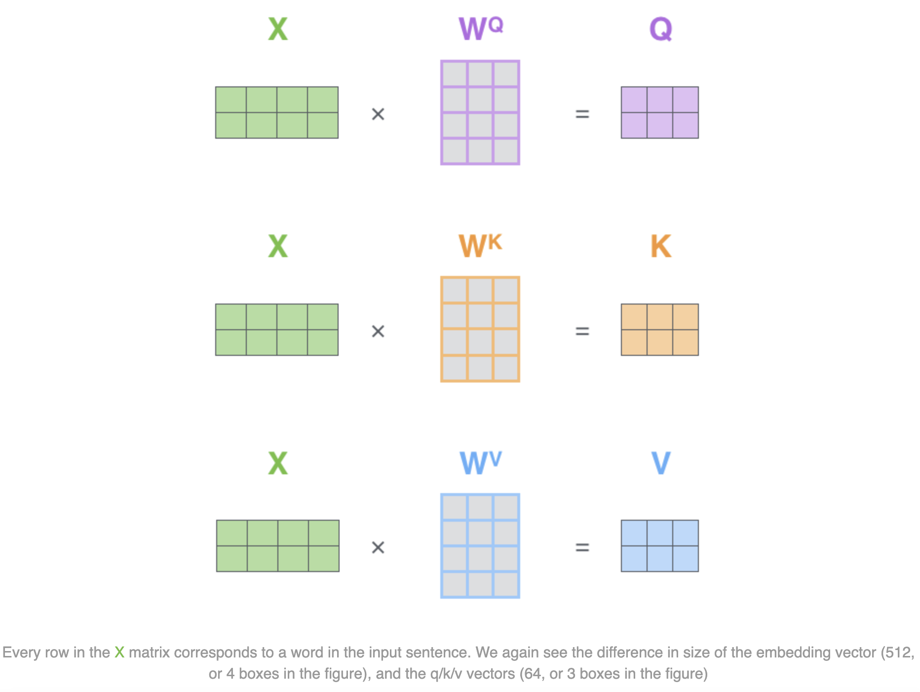
- For each word in the input sentence, the encoder computes three vectors called the "query", "key", and "value"
- These vectors are derived by multiplying the word's embedding with three trained weight matrices
- The weight matrices project the word embedding into the query, key, and value vector spaces, which are then used in the self-attention calculation
These vectors are smaller in dimension than the embedding vector: this is an architecture choice to make the
computation of multiheaded attention (mostly) constant
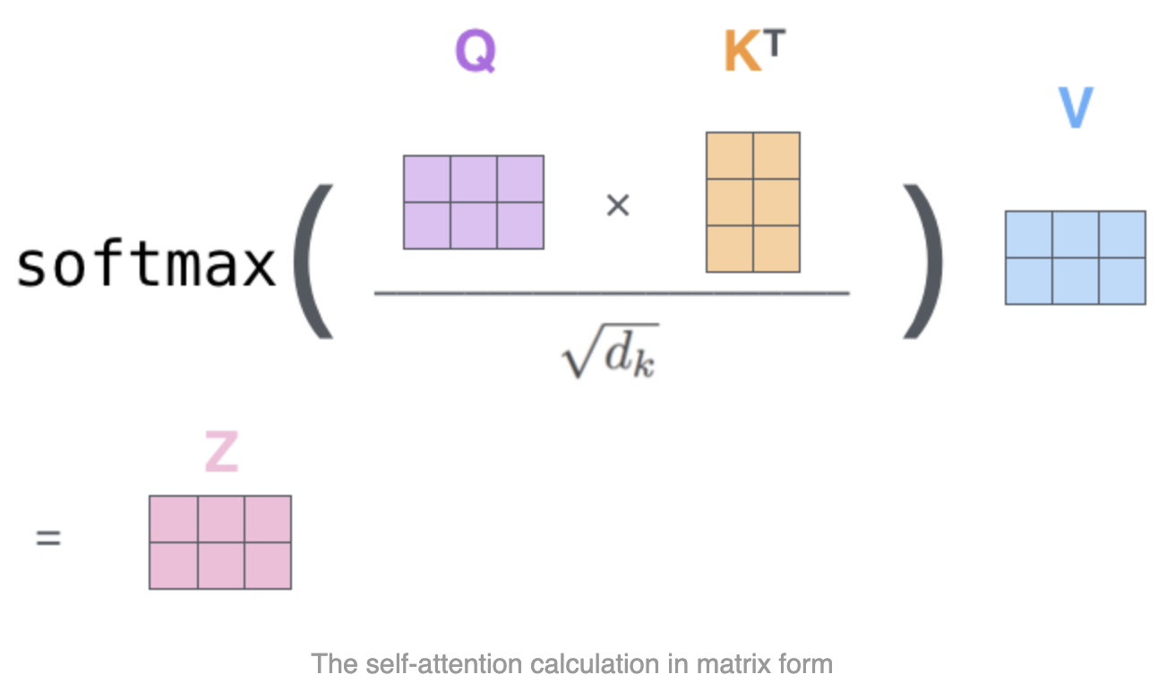
2. Calculate attention scores Q^K
- The attention scores determine how much importance or relevance to assign to other words in the input sentence when encoding the current word at a specific position
- To calculate the attention score between the current word and every other word, the model takes the dot product of the query vector for the current word and the key vector of the respective other word being scored against
- This operation is repeated for all word pairs in the sentence. It is parallielized using matrix multiplication where each row represents a word
- For instance, the attention scores for the word in position #1 will be [
q1^k1,q1^k2, …,q1^k64]
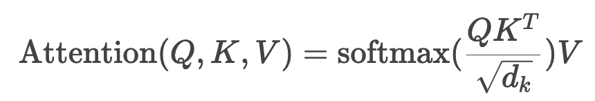
- The attention scores are divided by √64 = 8 (based on the dimension of the key vectors). This scaling helps stabilize the gradients during training
- The scaled scores are then passed through a softmax function to obtain normalized attention weights that sum to 1 across all words
- Each value vector is multiplied by its corresponding softmax attention weight
- The intuition here is to keep intact the values of the word(s) we want to focus on, and zero-out irrelevant words (by multiplying them by tiny numbers like 0.001, for example)
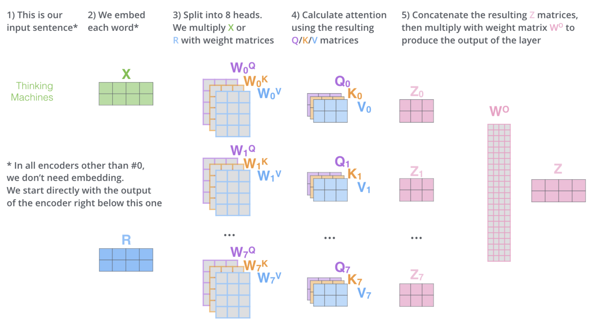
Multi-Head Attention
- Multi-head attention consists of several attention layers running in parallel, in attention heads
- It expands the model's ability to focus on different aspects of the input simultaneously by giving the attention block multiple "representation subspaces"
- The model can attend to different positional relationships and capture complementary context from various representation subspace
- We have multiple sets of query, key, value weight matrices in each attention head. Each set is used to project the input embeddings into a different representation subspace
- By combining the outputs, the model can integrate diverse contextual information and attend to a richer set of features when encoding each word
Positional Encoding
- The goal is to provide the model with information about the position and relative positions of words in the input sequence
- This is done by adding positional encoding vectors to the input word embeddings
- These vectors follow a specific pattern derived from sine and cosine functions of different frequencies, unique for each position
- By learning to associate these patterned vectors with word positions, the model can determine the order of words and the distances between them in the sequence
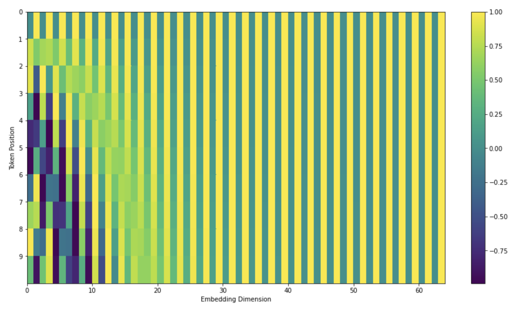
- The image represents a real example of positional encoding for 10 words (rows) with an hidden size of 64 (columns)
- The vectors exhibit an interleaved pattern because they are constructed by interweaving two signals
- One signal is generated using a sine function, where different frequency components (columns) follow a sinusoidal pattern across positions (rows)
- The other signal is generated using a cosine function, also with different frequency components (alternating columns) following a cosinusoidal pattern across positions
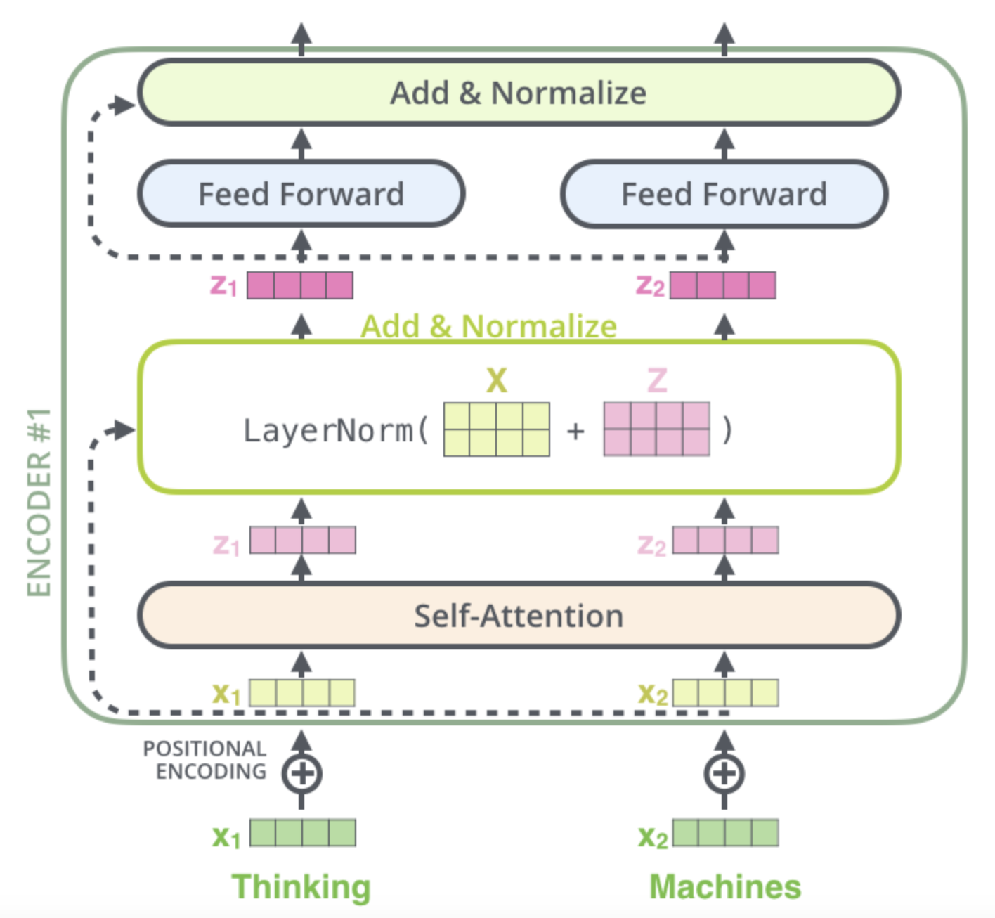
Residual connections
- The encoder and decoder components use residual connections followed by a layer normalization step
- The idea of residual connections is that every layer shouldn't create an entirely new type of representation,
replacing the old one with
x = layer(x). It should instead just tweak the existing representation with an update:x = x + layer(norm(x))
Decoder
- The blocks on the decoder side are similar to those on the encoder side
- Here's how they work together:
- The encoder takes in and processes the input sequence
- The top encoder's output is transformed into key (
K) and value (V) vectors - Each decoder block has an "encoder-decoder attention" layer that uses these
KandVvectors to focus on relevant parts of the input sequence while generating the output - For each step in the decoding phase:
- The decoder produces an output element based on the previous decoder output and the encoder representations
- The process repeats, with each decoder block attending to previous decoder outputs (via masked self-attention) and the encoder representations (via encoder-decoder attention)
- This continues until a special end-of-sequence symbol is generated
- Like the encoder, the decoder inputs are embedded and positionally encoded to incorporate sequential information
- However, in the decoder's self-attention, future positions are masked to prevent attending to subsequent outputs during prediction
- The "encoder-decoder attention" layer computes attention scores between the decoder's queries and the encoder's key-value pairs
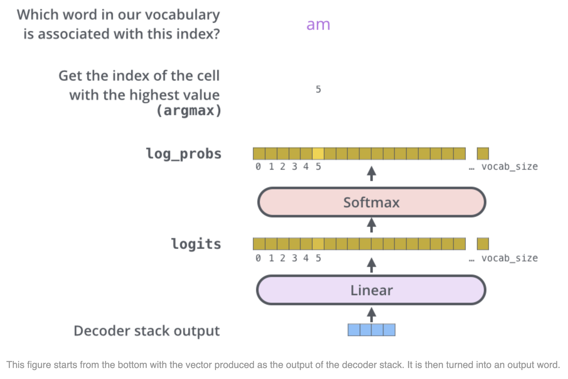
Final Linear and softmax layer
- The final linear layer is a fully connected neural network that projects the decoder's output vector into a larger logits vector with dimensionality equal to the vocabulary size
- Each element in the logits vector represents the score or prediction for a unique word in the vocabulary
- The softmax function is then applied to the logits vector to convert the scores into probabilities that sum to 1
- The word corresponding to the highest probability in the softmax output can be chosen as the predicted output for the current time step (greedy approach)
- Otherwise, the probability distribution can be used for Beam Search decoding to achieve a more sophisticated and higher-quality text generation!