🤝 Large-Scale Recommender Systems
Model vs System
- The role of a Recommender Model is scoring the interest a user may have with a set of items
- The scores represent the model's estimate of how interested a user will be in each item
- The role of a Recommender System is to scale the capabilities of one or more Recommender Model(s) to serve accurate and low-latency recommendations efficiently across various users, items, and scenarios
Recommendation Challenges
- Scalability: Scoring is computationally expensive. Item catalogues can grow to millions, hundreds of millions, even billions in extreme cases. Scoring every item for every user isn't feasible in most scenarios
- Cold-start problem: How to deal with new items and new users
- Online-offline gap: Live A/B results are not always correlated with offline experiments. It is difficult to estimate the dynamic effects of recommendations on user behavior and preferences, and live experiments can be costly and risky
- Freshness: Ideally, we want real-time recommendations, responsive to new items and the latest actions taken by users
- Noise: Data is often sparse and incomplete. We rarely obtain the ground truth of user satisfaction and instead model noisy implicit feedback signals. Furthermore, metadata associated with content is often poorly structured without a well-defined ontology
Evaluation
- During development, extensive use of offline metrics (precision, recall, ranking loss, etc.) is recommended to guide iterative improvements to the system
- However, for the final determination of the effectiveness of a model, A/B testing via live experiments is the gold standard
- Live experiments allow to measure subtle changes in click-through rate, and many other user engagement metrics
The Youtube paper illustrates the online-offline gap, showcasing how live experiments enabled the authors to iterate on their models and identify features that improved live metrics
Design Patterns
- To meet low-latency and high-precision serving requirements, large-scale recommenders are often deployed to production as multi-stage systems
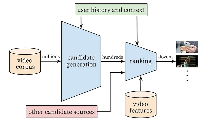
Traditional design pattern: 2-stage recommender system
1st stage: Candidate generation
- The first stage goal is to sift through >100M candidate items and retrieve a relevant ~hundreds subset for downstream ranking/filtering tasks
- Retrieval models requires efficiency: quickly evaluating more items per user increases the likelihood of finding the best, personalized item for them
- Multiple candidate sources within a single recommender system is common and ensure a diverse set of presented items to the user in the end
2nd stage: Ranking
- Objective: Optimize precision by re-ranking candidates
- Ranking models are generally more powerful, computationally expensive and heavyweight due to the lower number of items to score
- Ranking models benefit from a richer set of specialized features including candidate source information, scores assigned, users' previous interactions with the item and other similar items, etc.
- The ranking stage can be crucial for ensembling different candidate sources with non-comparable scores
Serving Diagram
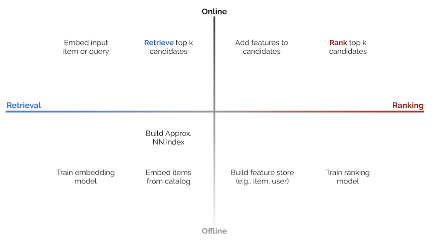
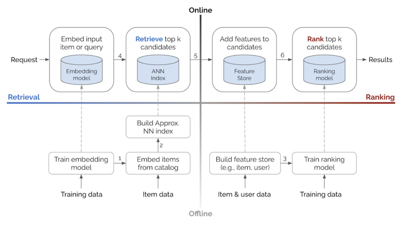
- Potential to efficiently recommend in real-time a larger corpus of items
- Improved performance within a fixed computational budget by splitting the tasks of recall and precision optimization between the candidate generator and ranker respectively, instead of having a single model trying to reach the best balance between both
- At the ranking step, it is possible to leverage very heavyweight models within the execution time constraints because the candidate set is significantly smaller
- Increased modeling flexibility and control over recommendations by stacking multiple specialized candidate generators, each targeting different aspects (e.g., exploration vs. exploitation)
☝️ Intuition: Given a catalog of 1 billion videos and a time constraint of 200 milliseconds to select a dozen videos for a user, you can only spend 0.2 nanoseconds per video for candidate selection. Within such a short timeframe, it's impossible to accurately compute a score for each video. Therefore, processing the videos in a multi-stage fashion allows you to achieve the best result within the given constraints by quickly selecting a relevant subset of items, and then taking more time to refine the selection
More advanced design pattern: 4-stage recommender system
- In practice, many items should be excluded from recommendations due to factors like unavailability, age restrictions, user history, licensing limitations, etc.
- Instead of relying on scoring or retrieval models to do this, a dedicated Filtering stage can be more helpful to enforce business rules in the recommender system
- Filtering can occur after Retrieval (with the challenge of ensuring enough candidates for Ranking), integrated with it, or after Ranking in some cases
- Filtering enables applying complex business logic rules that would be difficult or impossible for models to learn
- Examples include simple exclusion queries and more complex techniques like Bloom filters for removing previously interacted items
- Additionally, providing a diverse set of recommendations, including items outside the user's normal preferences, can help prevent filter bubbles and encourage exploration
- Having an explicit Ordering/Diversification stage can allow aligning model outputs with additional business needs or constraints
Revisited stages
1st stage: Candidate generation
- Same as previously
2nd stage: Filtering
- Apply business logic rules and filters to the retrieved candidate set
- Examples include excluding out-of-stock items, age-restricted content, previously consumed items, and items with licensing limitations
3rd stage: Ranking
- Same as previously
4th stage: Ordering/Diversification
- Provide a diverse set of recommendations, including items outside the user's normal preferences, to prevent filter bubbles and encourage exploration
- Align the final ranked list with additional business needs or constraints through an explicit ordering stage
Serving Diagram & Examples
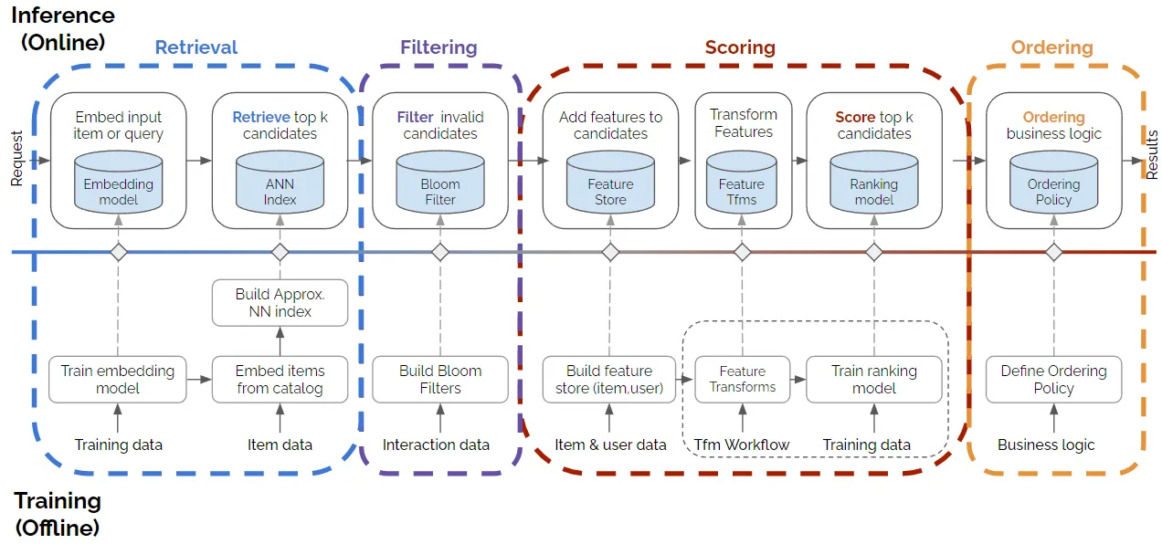
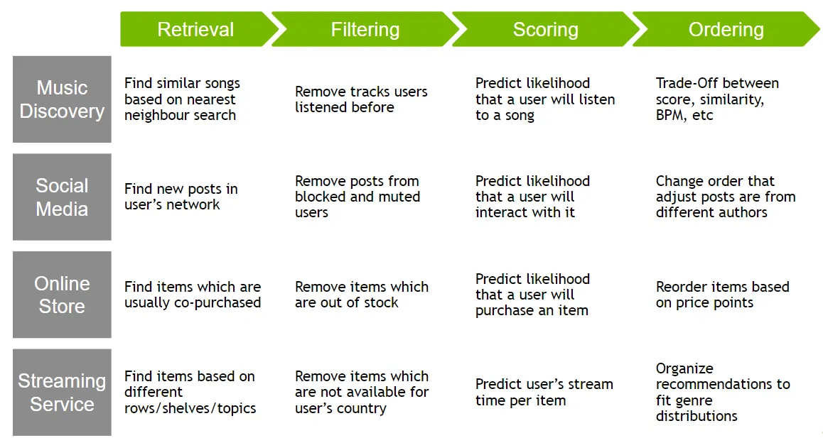
While more complicated, this system has the advantage of providing a more flexible and controllable way to enforce business rules and constraints in the recommendation process
Model Architectures
- Retrieval and Ranking models can take various forms, including matrix factorization, linear models, tree-models and neural networks
- In these notes, I'll delve deeper into two-tower models, a popular and effective approach that has gained prominence in recent years
- Two-tower models have gained popularity for their ability to efficiently handle retrieval tasks, but they can also be effectively applied to ranking tasks
- Notable examples of two-tower model usage include Google Play's retrieval, Instagram's Explore feature (with multi-task multi-label neural networks for ranking), Pinterest's, Expedia's, Snap's Spotlight, and Uber's recommendation system
What are Two-tower models?
- Two-tower models are part of neural deep retrieval (NDR), a latest modeling paradigm for retrieval
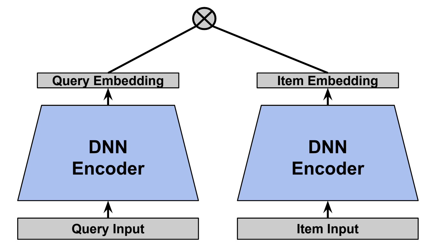
- A two-tower model consists of two separate neural networks, often referred to as "towers"
- Each tower processes query or item features to produce embedding representations, mapped to a shared vector space, allowing their similarities to be computed directly
- During training, the model learns to map queries and items to embeddings such that it maximizes the similarity between relevant pairs while minimizing similarity with irrelevant items
- Each tower learns layered representations of the input through successive network layers, transforming raw, multi-modal features to magnify useful information, filter out irrelevant data, and capture complex data relationships
Why use Two-tower models?
- Enhanced retrieval: Embedding-based methods outperform traditional keyword-based techniques (like inverted n-grams) by capturing semantic similarity rather than exact matches
- Flexible modeling: Decoupled query and item towers allow domain-specific feature selection and architectures, capturing complex, non-linear relationships in each domain
- Hybrid approach: Combine collaborative filtering (query-item interactions) with content-based filtering (entity features) for better recommendation quality and generalization
- Feature flexibility: Can leverage dense and sparse features (user profiles, historical engagements, metadata, context) for informative embeddings tailored to business goals
- Mitigate cold-start: Unlike factorization models, can generate meaningful embeddings for new items without user interactions using content features
- Efficient inference: Ability to decouple query and item inference
- Each tower only uses its respective input features to produce a vector, thereby the trained towers can be operationalized separately
- Decoupling inference of the towers for retrieval means we can precompute and cache vectors to reduce serving computation and latency
- It also means we can optimize each inference task independently
- Superior performance via expressivity and generalization
- Adaptability to diverse features and business objectives
- Reduced cold-start: Conceptually, we can think of a new candidate embedding compiling all the content-based and collaborative filtering information learned from candidates with the same or similar feature values
- Optimization opportunities for serving latency and compute
How to implement a Two-tower model?
Problem Formulation
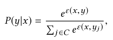
- Two-tower models treat the retrieval problem as a multi-class classification problem, where the likelihood of suggesting an item from a large corpus (classes) C is formulated as a softmax probability:
- Here, ε(x,y) is the logit (model output) for query x and item y, calculated as the inner product of their embeddings:
ε(x,y) = ⟨u(x; θ), v(y; θ)⟩
where u(x; θ) is the query embedding and v(y; θ) is the item embedding, both parameterized by θ
Data
- The YouTube paper emphasizes training a recommender on diverse examples, not just those produced by recommendations, to mitigate exploitation bias and quickly propagate user discoveries via collaborative filtering
- Another key insight that improved live metrics was to generate a fixed number of training examples per user to prevent highly active users from dominating the loss function
- Two-tower models typically use implicit engagement data to build positive user-item pairs and negative user-item pairs
- Implicit data is noisier but more voluminous than explicit feedback (often sparse), enabling deep-tail recommendations
- Missing interactions are considered potential negative signals (missing-as-negatives strategy), while interactions indicate positive signals
- User embeddings are learned from user history and context, which helps discriminate among items
- In practice, sampling negative user-item pairs is sufficient, as computing all would be computationally expensive (100x slower)
- There are two main approaches to efficiently implement negative sampling:
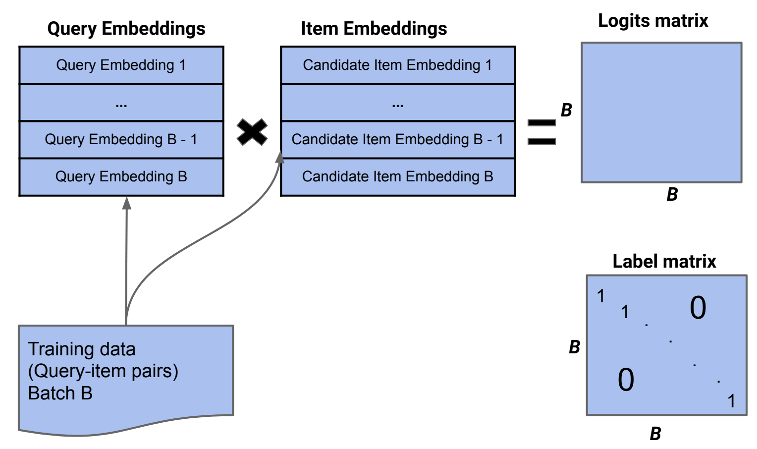
- In-batch negative sampling
- For a specific observation in a batch, consider every other observation in the same batch as negative
- This can lead to selection bias (biased softmax during training), mitigated by subtracting the log of item sampling probabilities (i.e., the log probability of that item occurring within the data) from logit scores (before softmax) during training to adapt the loss
- This technique is called log Q correction or sampled softmax in the literature
- Applying the correction significantly improves performance
- Without log Q correction, popular items are penalized as they appear more frequently as negatives during training, leading to underrecommendation and lower-quality suggestions
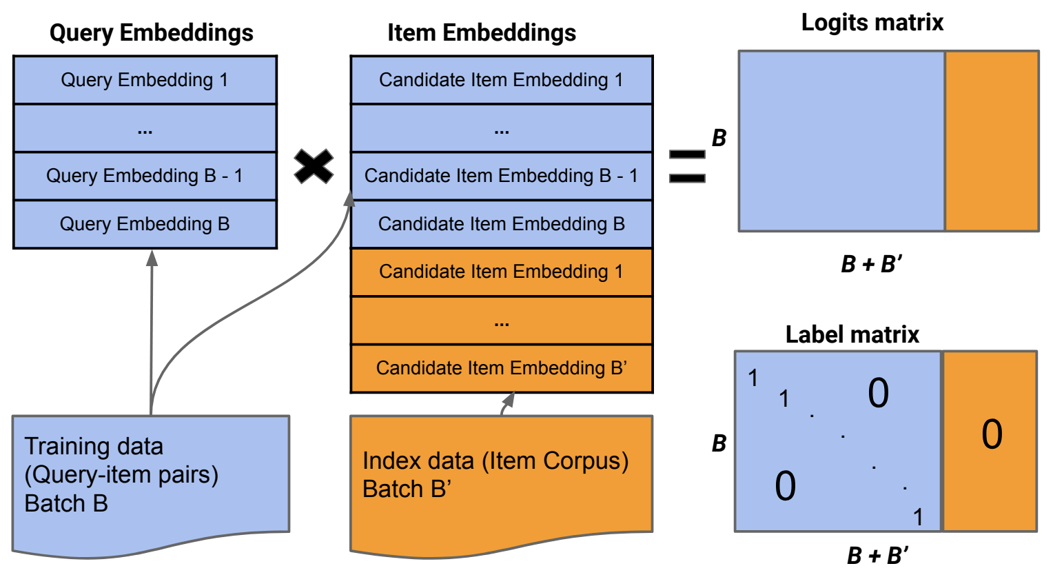
- Mixed Negative Sampling (MNS)
- Sample uniformly from all items to address the problem that in-batch sampled softmax never generates negatives from uninteracted items, penalizing and lacking resolution for unpopular, fresh or long-tail items
- Append zeros to the right of the label matrix to include non-interacted items in softmax
- MNS outperforms many baseline sampling methods by tackling selection bias in implicit user feedback
- Batch B' (a hyperparameter) contains items with no interaction with queries in batch B
- In practice, batch B' comes from an index with precomputed features; during training, each batch picks from this source
- Google's paper (2020) shows diminishing returns for B': larger B' improves results via larger sample size but may approximate uniform distribution beyond a certain point, deviating from serving time distribution and hurting performance. Also, increasing B' raises training costs, requiring a trade-off
- In-batch negative sampling
Feature Engineering
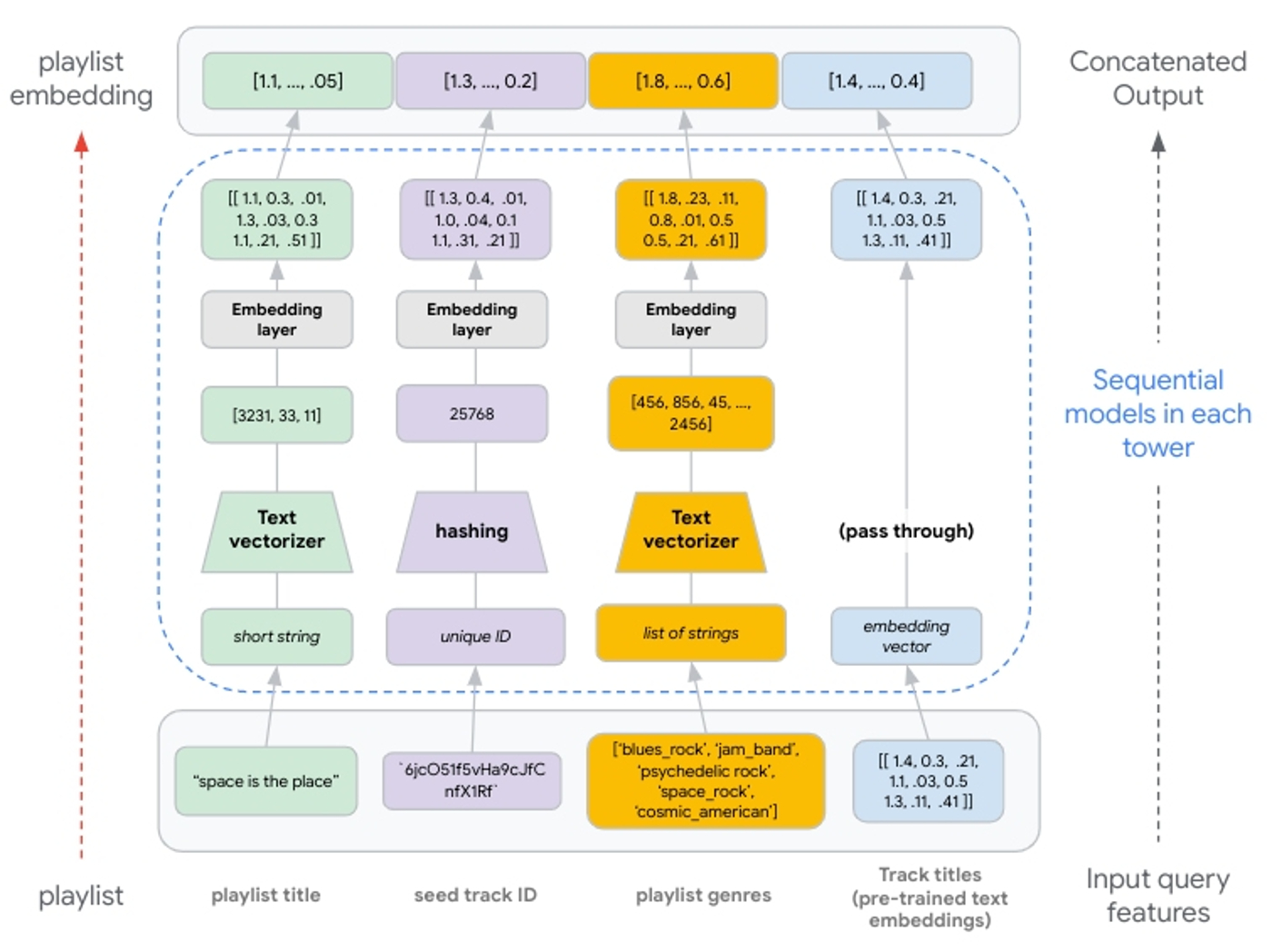
Overview- Two-tower models can handle multi-modal features (text, image, sound, etc.), sparse features and dense features
- These features are first converted into vector representations which can be concatenated and passed to subsequent model layers
- Text features: can be generated by using a text vectorizer if meaningful, or hashing otherwise
- Numeric features: can be normalized or discretized
- Pre-trained embeddings: can be directly used without transformation
- Normalizing continuous input features is crucial for neural network convergence; quantile normalization was used before training in the Youtube paper for instance
- Instead of preprocessing, some models apply transformations during training itself. For example, a batch normalization layer after numerical inputs can standardize them, as seen in TabNet. The DASALC model also uses raw features and applies transformations (Log, BN) during training, avoiding a separate preprocessing stage
- User activity data like purchase history and page views provides valuable input signals for building recommender models
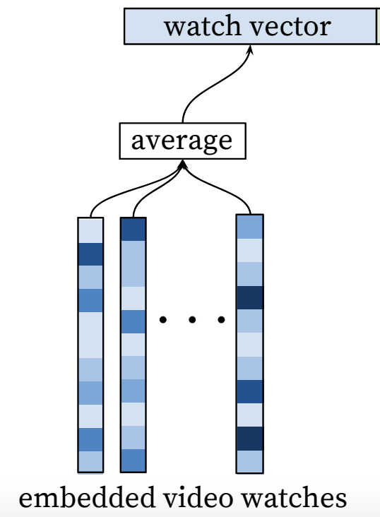
- However, users exhibit varying behavior, and activity is a sequence of events with different lengths across users. For instance, in the Youtube paper, a user's watch history is represented by a variable-length sequence of sparse video IDs
- To address this problem, sparse IDs can be mapped to dense vector representations via an embedding layer, learned jointly with all other model parameters. The network requires fixed-sized dense inputs, and the researchers found that averaging the embeddings performed best among other strategies (sum, component-wise max, etc.)
- The averaged embeddings of a user's activity (e.g. watched videos) can finally serve as a dense summary representation of their history
- Example: If User A watched 1 video and User B watched 3 videos, User A has 1 video embedding, while User B has 3. To obtain one fixed-sized input, concatenating embeddings isn't possible; instead, averaging allows for one embedding per user, with the same dimensionality as the video embeddings, regardless of the number of videos watched
- Demographic data provide priors for reasonable recommendations to new users
- User's geographic region and device information can be embedded and concatenated
- Binary (gender, login status) and continuous features (age) can be normalized between [0, 1(
- Item age: The Youtube paper showed that incorporating item age since availability improves recommendations for new and viral contents. Trained models can accurately capture time-dependant popularity patterns, avoiding an inherent bias towards older videos. This allows the recommendation system to prioritize recently uploaded videos that users are more likely to engage with, even if they don't have a large viewership history yet
- Frequency features: Features describing past item impressions are critical for introducing "churn" in recommendations, ensuring successive requests don't return identical lists. If a user was recently recommended an item but did not click/purchase it, then the model should naturally demote this item on the next page load
- Embedding strategy: Use the same underlying embedding for same categorical IDs to improve generalization, speed up training, and reduce memory requirements. For example, use the same embedding for video ID features (impression, last watched, seed) if they're all the same
- Super/sub-linear features: The YouTube paper found that adding squared and square-rooted versions of the normalized continuous features improved the model's expressive power. This allowed the network to easily model super-linear and sub-linear feature transformations. Providing these powered feature variants as inputs enhanced offline accuracy
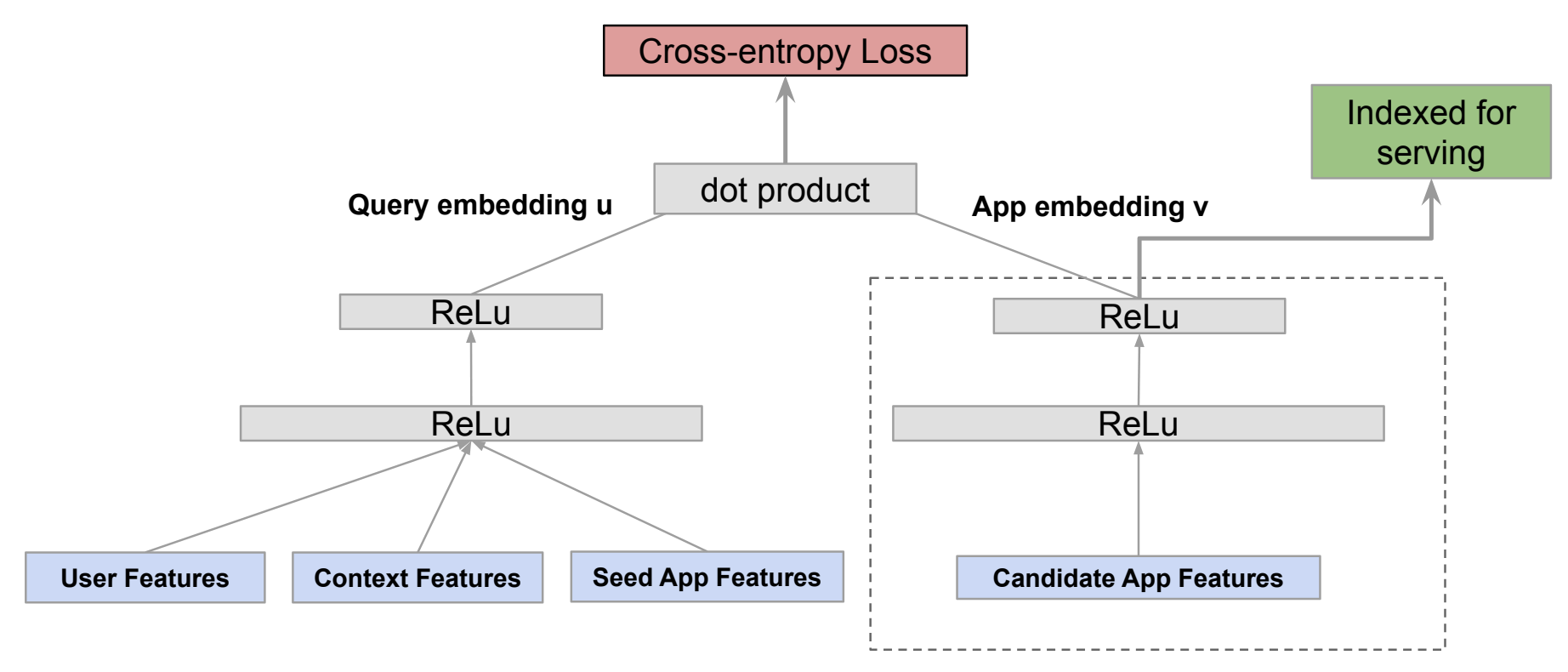
- Seed item: Seed item features can help predict next item preferences. For instance, seed app features help predict the next app installed for Google's Play
Model Architecture
Dense/MLP layers- Most popular and basic component of Two-tower models
- Adding more dense layers after concatenating embeddings can improve model expressiveness by allowing learning of successive feature representations
- The Youtube paper experimented with different depths to select the optimal number where diminishing returns appear
- Include cross layers after embeddings to explicitly model feature interactions before combining with dense layers that implicitly model interactions
- Cross layers often boost performance but increase computational complexity
- Evaluate parallel vs stacked implementations of cross and dense layers for best results
- Use self-attention to encode user history sequences, similar to word sequences
- Adding an L2 norm layer at the output can improve performance in some cases
- Relates to computing cosine similarity via dot product between final embeddings
Loss
- Cross entropy loss (or negative log likelihood)
Evaluation
- To avoid data leakage, use a temporal split to separate training and evaluation datasets. For example, train on 30 days of logged data and evaluate on the 31st day
- To account for seasonality, evaluations can be repeated over a rolling window and the results averaged. Example: To account for weekly patterns, train on a 30-day window, evaluating on day 31; then, repeat the evaluation 7 times, shifting the window by one day each time
- Retrieval models are typically optimized for recall and evaluated using Recall@K. This measures whether a relevant item is among the top K recommended items
Serving
- Model training: Train two-tower model offline, saving towers separately
- Item Tower deployment: Upload the trained item tower to a Model Registry
- Batch predictions: Run a GPU-accelerated batch job to precompute item embeddings
- Cache deployment: Compress item embeddings into an ANN (Approximate Nearest Neighbors) index optimized for low-latency retrieval, and deploy it to an endpoint for serving
- Query Tower deployment: Deploy trained query tower for real-time GPU-accelerated query embedding generation
- Search and retrieval: Use query embedding to retrieve the N nearest candidate embeddings from the index, then return product IDs using a Matching Engine
☝️ Note: For large item sets of millions or billions of vectors, nearest neighbor search is often a bottleneck for low-latency inference. ANN calculations optimize nearest neighbor search accuracy in a fraction of the time required for exhaustive searches. This is achieved through quantization-based hashing and tree search algorithms
Resources
- Mixed Negative Sampling for Learning Two-tower Neural Networks in Recommendations (Google paper, 2020)
- Recommender Systems, Not Just Recommender Models (NVIDIA Merlin, 2022)
- System Design for Recommendations and Search (by Eugene Yan, 2022)
- Scaling deep retrieval with Two-tower models (Google's Blog, 2023)
- Deep Dive: Softmax Approximation (Ruder, 2016)